Chapter 6 Data Quality
Before doing any analysis you must always check the data to ensure quality. Do not assume that because you are getting it from a source such as Yahoo! or Google that it is clean. I’ll show you why.
6.1 Yahoo! vs. Google
I’ll use dplyr 0.4.3, ggplot2 2.0.0 and tidyr 0.4.1 to help with analysis.
getSymbols("SPY",
           src = "yahoo",
           index.class = c("POSIXt", "POSIXct"),
           from = "2010-01-01",
           to = "2011-01-01",
           adjust = TRUE)
## [1] "SPY"yahoo.SPY <- SPY
summary(yahoo.SPY)## Index SPY.Open SPY.High
## Min. :2010-01-04 00:00:00 Min. :102.0 Min. :102.3
## 1st Qu.:2010-04-05 18:00:00 1st Qu.:108.0 1st Qu.:108.9
## Median :2010-07-04 00:00:00 Median :112.0 Median :112.7
## Mean :2010-07-03 16:28:34 Mean :112.8 Mean :113.5
## 3rd Qu.:2010-10-01 18:00:00 3rd Qu.:117.4 3rd Qu.:118.1
## Max. :2010-12-31 00:00:00 Max. :126.0 Max. :126.2
## SPY.Low SPY.Close SPY.Volume SPY.Adjusted
## Min. :100.1 Min. :101.1 Min. : 55309100 Min. : 90.81
## 1st Qu.:107.3 1st Qu.:108.2 1st Qu.:156667725 1st Qu.: 97.19
## Median :111.2 Median :112.0 Median :192116250 Median :100.59
## Mean :112.0 Mean :112.9 Mean :209692210 Mean :101.36
## 3rd Qu.:116.7 3rd Qu.:117.5 3rd Qu.:240310650 3rd Qu.:105.56
## Max. :125.9 Max. :125.9 Max. :647356600 Max. :113.07Above is a summary for the SPY data we received from Yahoo!. Examining each of the variables does not show anything out of the ordinary.
rm(SPY)
getSymbols("SPY",
           src = "google",
           index.class = c("POSIXt", "POSIXct"),
           from = "2010-01-01",
           to = "2011-01-01",
           adjust = TRUE)
## [1] "SPY"google.SPY <- SPY
summary(google.SPY)## Index SPY.Open SPY.High SPY.Low
## Min. :2010-01-04 Min. :103.1 Min. :103.5 Min. :101.1
## 1st Qu.:2010-04-05 1st Qu.:109.4 1st Qu.:110.4 1st Qu.:108.9
## Median :2010-07-04 Median :113.9 Median :114.5 Median :113.1
## Mean :2010-07-03 Mean :114.2 Mean :114.9 Mean :113.4
## 3rd Qu.:2010-10-01 3rd Qu.:118.4 3rd Qu.:119.0 3rd Qu.:117.8
## Max. :2010-12-31 Max. :126.0 Max. :126.2 Max. :125.9
## NA's :8 NA's :8 NA's :8
## SPY.Close SPY.Volume
## Min. :102.2 Min. : 0
## 1st Qu.:109.7 1st Qu.:151055510
## Median :113.8 Median :188064051
## Mean :114.2 Mean :203756549
## 3rd Qu.:118.5 3rd Qu.:239588977
## Max. :125.9 Max. :647356524
## Now we have a dataset from Google. it’s for the same symbol and same time frame. But now we have NA values - 8, in fact. In addition, our percentiles do not match up for any of the variables (with the exception of Date).
bind_rows(as.data.frame(yahoo.SPY) %>%
              mutate(Src = "Yahoo"),
          as.data.frame(google.SPY) %>%
              mutate(Src = "Google")) %>%
    gather(key, value, 1:4, na.rm = TRUE) %>%
    ggplot(aes(x = key, y = value, fill = Src)) +
    geom_boxplot() +
    theme_bw() +
    theme(legend.title = element_blank(), legend.position = "bottom") +
    ggtitle("Google vs. Yahoo! (non-NA)")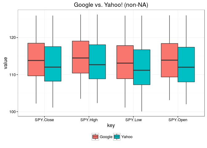
We can see above clearly we have a mismatch of data between Google and Yahoo!. For one reason, Google does not supply a full day of data for holidays and early sessions. Let’s look at the NA values:
as.data.frame(google.SPY) %>%
    mutate(Date = index(google.SPY)) %>%
    select(Date, starts_with("SPY"), -SPY.Volume) %>%
    filter(is.na(SPY.Open))
## Date SPY.Open SPY.High SPY.Low SPY.Close
## 1 2010-01-15 NA NA NA 113.64
## 2 2010-02-12 NA NA NA 108.04
## 3 2010-04-01 NA NA NA 117.80
## 4 2010-05-28 NA NA NA 109.37
## 5 2010-07-02 NA NA NA 102.20
## 6 2010-09-03 NA NA NA 110.89
## 7 2010-11-24 NA NA NA 120.20
## 8 2010-12-23 NA NA NA 125.60We can see many of these dates correspond closely to national holidays; 2010-11-24 would be Thanksgiving, 2010-12-23 would be Christimas.
So where Yahoo! does give OHLC values for these dates, Google just provides the Close. This won’t affect most indicators that typically use closing data (moving averages, Bollinger Bands, etc.). However, if you are working on a strategy that triggers a day prior to one of these holidays, and you issue a buy order for the next morning, this may cause some integrity loss.
This doesn’t mean you should only use Yahoo!. At this point we don’t know the quality of Yahoo!’s data - we only know it seems complete. And this may be enough depending on what you want to do.
However, it’s up to you to ensure your data is top quality.
Garbage in, garbage out
6.2 Examining Trades
It’s not just data that we want to QA against but also our trades. After all, how disappointing would it be to think you have a winning strategy only to learn you were buying on tomorrow’s close instead of today (look-ahead bias). Or that you wrote your rules incorrectly?
Every backtest must be picked apart from beginning to end. Checking our data was the first step. Checking our trades is next.
We’ll reload our Luxor strategy and examine some of the trades for SPY.
rm.strat(portfolio.st)
rm.strat(account.st)
symbols <- basic_symbols()
getSymbols(Symbols = symbols, src = "yahoo", index.class = "POSIXct",
           from = start_date, to = end_date, adjust = adjustment)
initPortf(name = portfolio.st, symbols = symbols, initDate = init_date)
initAcct(name = account.st, portfolios = portfolio.st, initDate = init_date,
         initEq = init_equity)
initOrders(portfolio = portfolio.st, symbols = symbols, initDate = init_date)
applyStrategy(strategy.st, portfolios = portfolio.st)
checkBlotterUpdate(portfolio.st, account.st, verbose = TRUE)
updatePortf(portfolio.st)
updateAcct(account.st)
updateEndEq(account.st)chart.Posn(portfolio.st, Symbol = "SPY", Dates="2008-01-01::2008-07-01",
TA="add_SMA(n = 10, col = 2); add_SMA(n = 30, col = 4)")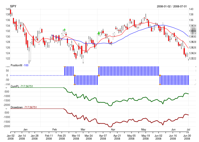
Figure 6.1: SPY Trades for Jan 1, 2008 to July 1, 2008
Our strategy called for a long entry when SMA(10) was greater than or equal to SMA(30). It seems we got a cross on February 25 but the trade didn’t trigger until two days later. Let’s take a look.
le <- as.data.frame(mktdata["2008-02-25::2008-03-07", c(1:4, 7:10)])
DT::datatable(le,
              rownames = TRUE,
              extensions = c("Scroller", "FixedColumns"),
              options = list(pageLength = 5,
                             autoWidth = TRUE,
                             deferRender = TRUE,
                             scrollX = 200,
                             scroller = TRUE,
                             fixedColumns = TRUE),
              caption = htmltools::tags$caption(
                  "Table 6.1: mktdata object for Feb. 25, 2008 to Mar. 7, 2008"))
The 2008-02-25T00:00:00Z bar shows nFast just fractions of a penny lower than nSlow. We get the cross on 2008-02-26T00:00:00Z which gives a TRUE long signal. Our high on that bar is $132.61 which would be our stoplimit. On the 2008-02-27T00:00:00Z bar we get a higher high which means our stoplimit order gets filled at $132.61. This is reflected by the faint green arrow at the top of the candles upper shadow.
ob <- as.data.table(getOrderBook(portfolio.st)$Quantstrat$SPY)
DT::datatable(ob,
              rownames = FALSE,
              filter = "top",
              extensions = c("Scroller", "FixedColumns"),
              options = list(pageLength = 5,
                             autoWidth = TRUE,
                             deferRender = TRUE,
                             scrollX = 200,
                             scroller = TRUE,
                             fixedColumns = TRUE),
              caption = htmltools::tags$caption(
                  "Table 6.2: Order book for SPY"))
## Warning in min(d, na.rm = TRUE): no non-missing arguments to min; returning
## Inf## Warning in max(d, na.rm = TRUE): no non-missing arguments to max; returning
## -InfWhen we look at the order book (Table 6.2) we get confirmation of our order. index reflects the date the order was submitted. Order.StatusTime reflects when the order was filled.
(Regarding the time stamp, ignore it. No time was provided so by default it falls to midnight Zulu time which is four to five hours ahead of EST/EDT (depending on time of year) which technically would be the previous day. To avoid confusion, just note the dates.)
If we look at Rule we see the value of EnterLONG. These are the labels of the rules we set up in our strategy. Now you can see how all these labels we assigned earlier start coming together.
On 2008-03-06T00:00:00Z we get a market order to vacate all long positions and take a short positions. We see this charted in Fig. 6.1 identified with a red arrow on the same candle one bar after the cross. We stay in that position until 2008-04-01T00:00:00Z when we flip back long.
If you flip to page 5 of Table 6.2, on 2009-11-03T00:00:00Z you will see we had an order replaced (Order.Status). Let’s plot this time frame and see what was going on.
chart.Posn(portfolio.st, Symbol = "SPY", Dates="2009-08-01::2009-12-31",
           TA="add_SMA(n = 10, col = 2); add_SMA(n = 30, col = 4)")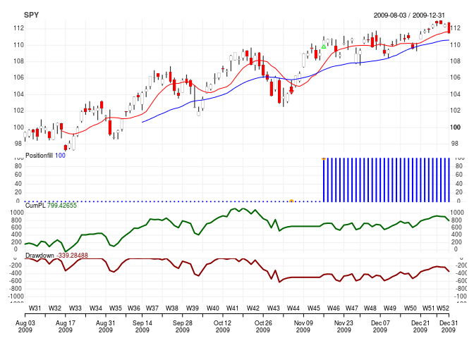
Figure 6.2: SPY Trades for Jan 1, 2008 to July 1, 2008
We got a bearish SMA cross on November 2 which submitted the short order. However, our stoplimit was with a preference of the Low and a threshold of $0.0005 or $102.98. So the order would only fill if we broke below that price. As you see, that never happened. The order stayed open until we got the bullish SMA cross on Nov. 11. At that point our short order was replaced with our long order to buy; a stoplimit at $109.50. Nov. 12 saw an inside day; the high wasn’t breached therefore the order wasn’t filled. However, on Nov. 13 we rallied past the high triggering the long order (green arrow). This is the last position taken in our order book.
So it seems the orders are triggering as expected.
On a side note, when I was originally writing the code I realized my short order was for +100 shares instead of -100 shares; actually, orderqty = 100 which meant I wasn’t really taking short positions.
This is why you really need to examine your strategies as soon as you create them. Before noticing the error the profit to drawdown ratio was poor. After correcting the error, it was worse. It only takes a minor barely recognizable typo to ruin results.
Finally, we’ll get to the chart.Posn() function later in the analysis chapters. For now I want to point out one flaw (in my opinion) with the function. You may have noticed our indicators and positions didn’t show up immediately on the chart. Our indicators didn’t appear until the 10-bar and 30-bar periods had passed. And our positions didn’t show up until a new trade was made.
You may also notice our CumPL and Drawdown graphs started at 0 on the last chart posted.
chart.Posn() doesn’t “zoom in” as you may think. Rather it just operates on a subset of data when using the Dates parameter. Effectively, it’s adjusting your strategy to the Dates parameter that is passed.
chart.Posn(portfolio.st, Symbol = "SPY",
           TA="add_SMA(n = 10, col = 2); add_SMA(n = 30, col = 4)")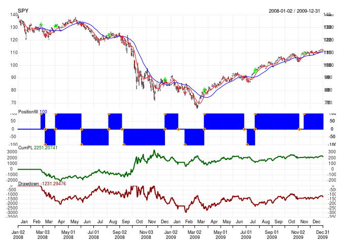
Figure 6.3: SPY Trades for Jan 1, 2008 to July 1, 2008
Also, note the CumPL value of $2251.20741 and Drawdown value of -$1231.29476 are the final values. It does not show max profit or max drawdown. Notice the values are different from figure 6.3 and figure 6.2.
Going by that alone it may seem the strategy overall is profitable. But when you realize max drawdown was near -$3,000 and max profit was up to $3,000, it doesn’t seem so promising.
Again, we’ll get into all of this later. Just something to keep in mind when you start doing analysis.