Chapter 11 Obtaining Resources
Some of you may not have the resources needed to run complex strategies. Some of you may have dual or quad core processors (even more) but still find some strategies taking a bit of time to run. Nothing is worse than running a strategy for ten or thirty minutes or even longer to find something’s not right. This can get more irritated if you’re running on a large number of symbols.
11.1 Amazon Web Services
Amazon Web Services is a cloud-computing service that allows us to use resources that may not normally be available to us. They’re are literally dozens of services available depending on your needs.
The one we will focus on here is EC2 or Elastic Compute Cloud. EC2 offers virtual server space in the Linux and Windows platforms. With EC2 we can get a very minimal setup for as little as $0.006 per hour.
You do not need to have this service running 24 hours a day. One of the huge benefits of the service is we only need to fire it up when we’re ready to do something. It takes just a few minutes to boot up. We only pay for uptime.
Another advantage is we can use multiple instances. We can have one server testing a script or running an analysis and work on the same project on another server.
In addition, if you’ve never used Amazon Web Services before you are likely available for a one year free trial. There may be some restrictions. With the free trial you can get the t2.micro service which gives 1GB of memory and a 1 core 2.40Ghz processor, leave it running 24 hours a day, 7 days a week for a full year and not pay a dime. This is plenty to get the basic foundation layed.
When you see this block it means we are going to perform some operations that may incur a charge depending on your AWS account. It is up to you to know the associated costs for your account.
We’re also going to take advantage of a tremendous service offered by Louis Aslett. Louis has taken the time to create and maintain dozens of Linux images set up with RStudio. Don’t worry if you’re not familiar with Linux. After the initial setup you’ll rarely need it.
11.2 Getting Started
If you have not used AWS before go create an account. Registration takes just a few minutes.
When finished, we’ll go to Louis Aslett’s website to grab an image.
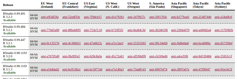
You’ll see the RStudio/R images listed down the left side and server locations across the header. You want to find the server location closest to you but for our purposes it shouldn’t matter much. The latest release as of this writing that is RStudio 0.99.491 with R 3.2.3 (This book is written in RStudio 0.99.893 using R 3.2.3).
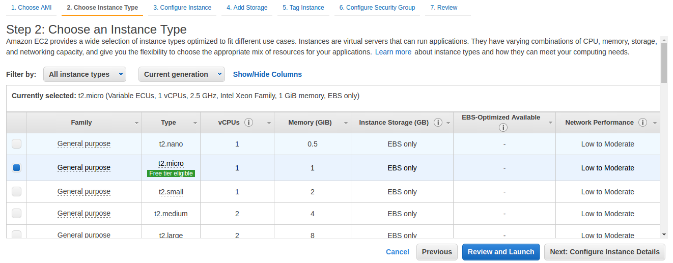
Click on the corresponding ami hyperlink. This will take you to choose an instance type. If you’re eligible for the free-tier service you’ll see the green font accent beneath the t2.micro service.
Click “Next: Configure Instance Details” and keep clicking Next until you get to Step 6: Configure Security Group. By default port 22 is open for SSH from any IP address. You can close this if you like. However, I like to install my R libraries to the root user through SSH. I’ll demonstrate this later. If you choose to keep SSH change Source to Custom IP and your IP address range should pop up in the text field to the right.
You also want to click “Add Rule” to open port 80. Select the “Custom TCP Rule” under Type and change it to HTTP. This will add the value 80 under Port Range. As with SSH change Source to Custom IP and again your IP address range will automatically fill in.
You can also create your own Security group name or leave the default. I used rstudio-0-99-491.
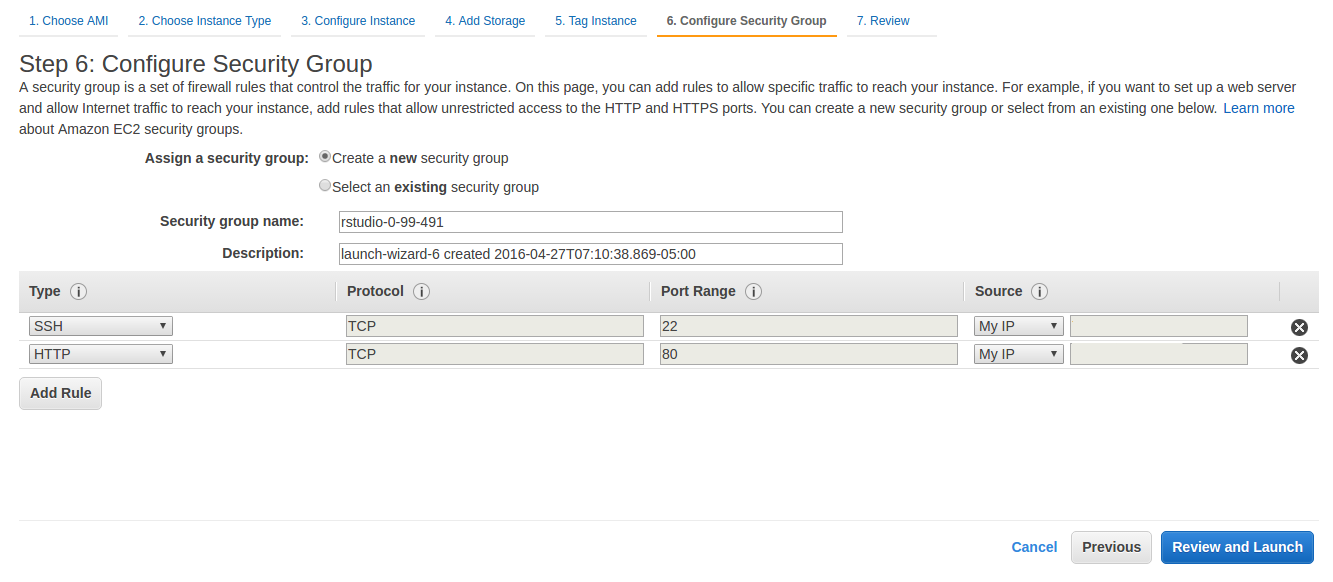
Do not leave Source open to “Anywhere” as this will allow anyone to potentially attempt to access your virtual server. This may seem harmless but if you’re working solo there’s no sense having it all open unless you’re comfortable with Linux security. If you’re working in groups, use Github.
Next, click “Review and Launch”. This will take you to a summary page reiterating your selections. If all looks good click “Launch”.
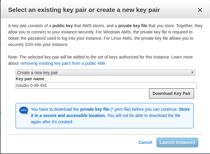
If you left SSH open you’re not quite done yet. You’ll see a pop-up window asking you to create or use an existing key pair. A private key is used to SSH into your remote server. Select “Create a new key pair” from the drop down menu and give a Key pair name; I named mine after my security group for simplicity. Click “Download Key Pair” and save the pem file to a safe location. When you’ve saved the pem file click “Launch Instances”.
If you’re service is running but you are unable to log in via SSH or HTTP it is likely because your IP address has been changed by your DNS provider. See Adding Rules to a Security Group on changing the IP rules.
Once you launch an instance you are now on the billing clock. If you were eligible for the free-tier and selected the t2.micro instance you should not be incurring charges during your trial.
While you are waiting, if you are on a Windows system and left SSH enabled please take a moment to review Connecting to Your Linux Instance from Windows Using PuTTY. You will need to convert the pem file to a ppk file in order to log in.
As we wait you’ll notice Instance State is listed as “running” but Status Checks shows as “initializing”. Once Status Checks displays “2/2 checks…” you are now ready to log in to your new server.
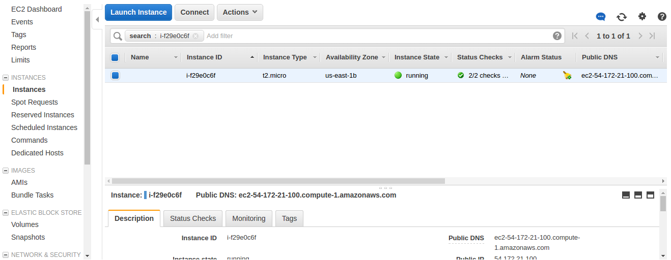
Take a look at the frame in the bottom of your browser. You’ll see your instance ID followed by Public DNS. Copy the Public DNS and paste it into a new browser window or tab and hit enter. You should now be greeted by a RStudio login page. Congratulations!
We’re not done yet. The default username and login to the AMI is rstudio for both Username and Password. So go ahead and log into your system. When RStudio loads you will see a commented script in the editor. Read over it carefully and follow the instructions particularly in regards to changing your password. I would suggest getting a new password from Secure Password Generator. The defaults should suffice. After running passwd() you should get a confirmation message:
(current) UNIX password: Enter new UNIX password: Retype new UNIX password: passwd: password updated successfully
You are now set up to use RStudio as you have been.
11.2.1 Installing Quantstrat
If you attempt to install quantstrat from the RStudio package window or from Cran you will get an error that it is not available for R 3.2.3. You can install it from R-Forge.
install.packages("quantstrat", repos="http://R-Forge.R-project.org")This will install the latest version, 0.9.1739, the same as used in this book along with the additional libraries needed.
11.3 Testing Resources
We’ll use a minor variation of the MACD demo in quantstrat to test some speeds. The strategy will buy when our signal line crosses over 0 and sell when it crosses under 0.
We’ll use a range of 1:20 for fastMA and 30:80 for slowMA. The original demo called for a random sample of 10 but we’ll remove that to test all 1,020 iterations.
We will execute the strategy on one stock, AAPL, from 2007 to Jun. 1, 2014.
These tests are performed using Ubuntu 14.04.3 LTS, x86 64 bit.
The unevaluated code is as follows:
start_t <- Sys.time()

library(quantstrat)
# For Linux
library(doMC)
registerDoMC(cores = parallel::detectCores())

stock.str <- "AAPL" # what are we trying it on

#MA parameters for MACD
fastMA <- 12
slowMA <- 26
signalMA <- 9
maType <- "EMA"
.FastMA <- (1:20)
.SlowMA <- (30:80)

currency("USD")
stock(stock.str, currency = "USD", multiplier = 1)

start_date <- "2006-12-31"
initEq <- 1000000
portfolio.st <- "macd"
account.st <- "macd"

rm.strat(portfolio.st)
rm.strat(account.st)

initPortf(portfolio.st, symbols = stock.str)
initAcct(account.st, portfolios = portfolio.st)
initOrders(portfolio = portfolio.st)

strat.st <- portfolio.st
# define the strategy
strategy(strat.st, store = TRUE)

#one indicator
add.indicator(strat.st,
              name = "MACD",
              arguments = list(x = quote(Cl(mktdata)),
                               nFast = fastMA,
                               nSlow = slowMA),
              label = "_")

#two signals
add.signal(strat.st,
           name = "sigThreshold",
           arguments = list(column = "signal._",
                            relationship = "gt",
                            threshold = 0,
                            cross = TRUE),
           label = "signal.gt.zero")

add.signal(strat.st,
           name = "sigThreshold",
           arguments = list(column = "signal._",
                            relationship = "lt",
                            threshold = 0,
                            cross = TRUE),
           label = "signal.lt.zero")

# add rules

# entry
add.rule(strat.st,
         name = "ruleSignal",
         arguments = list(sigcol = "signal.gt.zero",
                          sigval = TRUE,
                          orderqty = 100,
                          ordertype = "market",
                          orderside = "long",
                          threshold = NULL),
         type = "enter",
         label = "enter",
         storefun = FALSE)

# exit
add.rule(strat.st,
         name = "ruleSignal",
         arguments = list(sigcol = "signal.lt.zero",
                          sigval = TRUE,
                          orderqty = "all",
                          ordertype = "market",
                          orderside = "long",
                          threshold = NULL,
                          orderset = "exit2"),
         type = "exit",
         label = "exit")

### MA paramset

add.distribution(strat.st,
                 paramset.label = "MA",
                 component.type = "indicator",
                 component.label = "_", #this is the label given to the indicator in the strat
                 variable = list(n = .FastMA),
                 label = "nFAST")

add.distribution(strat.st,
                 paramset.label = "MA",
                 component.type = "indicator",
                 component.label = "_", #this is the label given to the indicator in the strat
                 variable = list(n = .SlowMA),
                 label = "nSLOW")

add.distribution.constraint(strat.st,
                            paramset.label = "MA",
                            distribution.label.1 = "nFAST",
                            distribution.label.2 = "nSLOW",
                            operator = "<",
                            label = "MA")


getSymbols(stock.str, from = start_date, to = "2014-06-01")

results <- apply.paramset(strat.st,
                          paramset.label = "MA",
                          portfolio.st = portfolio.st,
                          account.st = account.st,
                          nsamples = 0,
                          verbose = TRUE)

updatePortf(Portfolio = portfolio.st,Dates = paste("::",as.Date(Sys.time()),sep = ""))
end_t <- Sys.time()
print(end_t-start_t)
servers <- c("t2.micro", "t2.medium", "m4.xlarge", "m4.2xlarge", "m4.4xlarge")
aws <- data.frame("Server" = factor(servers, levels = servers),
"Processor" = c("Intel Xeon E5-2676 v3, 2.40 GHz",
"Intel Xeon E5-2670 v2, 2.50 GHz",
"Intel Xeon E5-2676 v3, 2.40Ghz",
"Intel Xeon E5-2676 v3, 2.40Ghz",
"Intel Xeon E5-2676 v3, 2.40Ghz"),
"VirtualCores" = c(1, 2, 4, 8, 16),
"Memory" = c(1, 4, 16, 32, 64),
"Seconds" = c(749.841, 293.6499, 118.1366, 62.24196, 34.68986),
"Price" = c(0.013, 0.052, 0.239, 0.479, 0.958))
# knitr::kable(aws, caption = "Test Results for AWS", booktabs = TRUE)aws %>%
ggplot(aes(x = Server, y = Seconds, fill = Server)) +
geom_bar(stat = "identity") +
theme_bw() +
labs(title = "Execution Time per Server")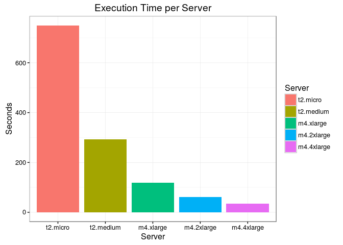
aws_ppe <- aws %>%
    mutate(ppe = (Price/60) * Seconds)

aws_ppe %>%
    ggplot(aes(x = Server, y = ppe, fill = Server)) +
    geom_bar(stat = "identity") +
    theme_bw() +
    labs(title = "Cost per Second of Execution (ppe)", y = "Cost (USD)")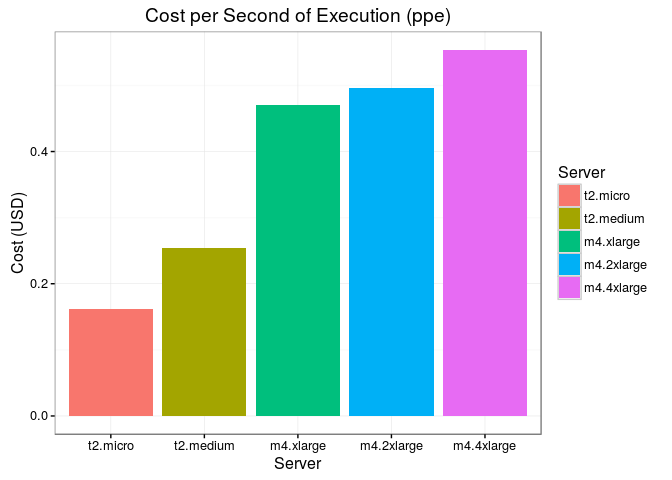
# knitr::kable(aws_ppe, caption = "Cost per Second of Execution (ppe)",
#              y = "Cost (USD)", booktabs = TRUE)
We can get a general idea of costs by comparing execution times versus the cost of the server. Keep in mind this may vary by script and using other servers available.
Obviously we’re paying a premium for speed though all things considered there isn’t much of a difference going from m4.xlarge to m4.4xlarge. Prices are not prorated for hourly usage so if you’re going to pay a premium for the faster servers it may not be a bad idea to have several backtests ready to run.
11.4 Changing Instances
Regardless if you’re free-tier eligible or not, using any server instance beyond the t2.micro will incur charges. See Amazon EC2 Pricing for more details.
To change your instance types go to your EC2 Dashboard then click the Instances link under Instances. Check the box next to your instance then click on the Actions dropdown.
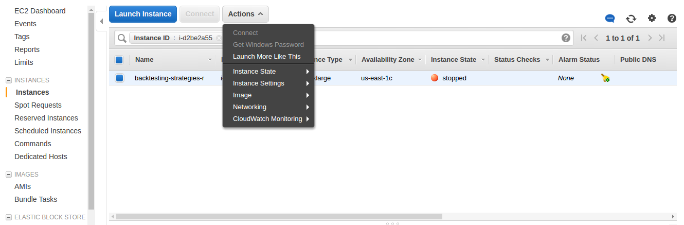
If your instance is already running stop it by selecting Instance State > Stop.
With the instance stopped under Instance State go back to Actions and select Instance Settings > Change Instance Types. Then select your instance from the select field and Apply.
You can restart the instance right away by going back to Actions > Instance State > Start. It will take a few minutes but will be ready to go when Status Checks reads “2/2 checks…”.
11.5 Stop the Server
Do not terminate the server else you will lose all of your data. There is no charge for stopping an instance and it only takes minutes to fire it back up when you’re ready to work.
When you finish your workload be sure to log off RStudio. You can stop the instance by going to Actions > Instance State > Stop. All of your data will be saved for the next time you are ready to work.
When you stop/start or restart a server you will receive a new Public DNS. If you have stored your original Public DNS as a bookmark or in PuTTY, be sure to update it to the new DNS assigned by AWS when the server is started. You can use Elastic IPs to keep a consistent IP address. However, this is only free if you leave your instance running 24/7.
After you have stopped the server you are no longer incurring charges regardless of the instance type. However, you may want to downgrade the Instance Type to be safe the next time you start the server.
11.6 Reading Resources
If you are interested in further utilizing AWS for your backtesting I recommend the book Amazon Web Services in Action (affiliate link) by Andreas and Michael Wittig. The book details virtual hosting and storage services as well as proper security. If you intend to develop complex strategies in R but lack the resources you may find AWS can be a great option.
If you’re going to use Ubuntu I would also recommend The Official Ubuntu Server Book (affiliate link) by Kyle Rankin and Benjamin Mako Hill.